
In previous posts, we discussed magnetic recording. Here, we extend this discussion by looking at the effect of a thermal bath that is coupled to magnetic moments during recording.
Once again, we start with the Landau-Lifshitz-Gilbert (LLG) equation

where  is an unit vector describing the orientation of the magnetic moment,
  is time,
  is the gyromagnetic ratio,
  is the effective field and
  is a damping constant. Landau added the second term in order that the magnetization moment would come into equilibrium (e.g.
  and therefore
  ) eventually. The equation has been derived in multiple theories for particular cases. In particular, [1] recovered LLG from a quantum macrospin in the limit of constant coupling and uniform density of states of the thermal bath.
For small magnetic particles, Brown [2] derived the required stochastic field from the Fokker-Planck equation. The resulting stochastic field,  , is a Gaussian with mean of zero and variance,
  in each dimension where
  is temperature,
  is the saturation magnetization and
  is the volume of the magnetic grain.
The stochastic field will cause a diffusion of from its equilibrium. Then, since  the precession term will introduce a rotational flux of . Ignoring this rotational flux, we can define a diffusion coefficient of the magnetization as

where the last equality is calculated by replacing with Brown’s stochastic fields in the LLG and integrating over all . Reasonable values would give  rad
rad /s. Roughly speaking this would mean in 1ns would have diffused ~
 –
–  from equilibrium. This does not include the additional processional term which also depend on this angle.
Instead of diffusion of magnetization, one could look at diffusion of free energy,  , of the magnetic moment. In this case,

and one can show Einstein’s relation holds,  , where
  is advective flux due to
  in the absence of stochastic fields, namely
 .
.
From above, any analysis should include since it’s a consequence of damping ( ). We will show its effect during conventional magnetic recording.
For conventional writing, as discussed previously, the applied write field goes as  such that
  is a slowly varying function of time (i.e. medium motion). On the other hand,
  is quickly varying in ~ 0.1ns with a peak large enough to eliminate the free energy barrier (e.g
 ![H_a > \left[H_k - (3 N /2 - 2\pi)M_{s_i}\right] / 2](https://entonos.com/wp-content/ql-cache/quicklatex.com-0289130fe6461e41f288404156ae6485_l3.png "Rendered by QuickLaTeX.com") ). Therefore, one would expect the diffusive flux (e.g.
). Therefore, one would expect the diffusive flux (e.g.  ) would lower required
  .
.
We first confirm does, in fact, result in a Boltzmann distribution of the orientation of .
For micro-magnetic simulations, we have identical square prisms (extruded 10nm) grains of volume 503nm packed in a periodic square lattice with
  kOe,
kOe,  (
( ) is normal to media plane,
  emu/cc and
  .
.
For simplicity, we take 65536 grains,  K and exclude applied and magnetostatic fields. We start with all the grains along and integrate in time until equilibrium is achieved.
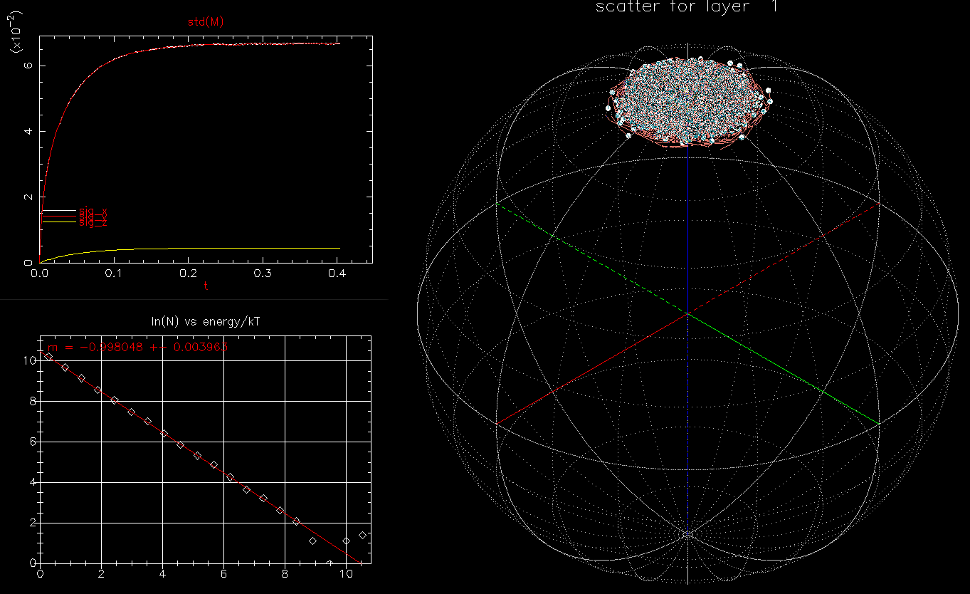
 . Upper left, standard deviation of
  and
and  as a function of time (ns); lower left, histogram of as a function of energy
 ; right, isometric projection of all grain orientations on a unit sphere: each white circle represents one magnetic orientation with orange trail showing short time history of orientation.
We see not only is the standard deviation of is as expected at equilibrium but the time evolution to equilibrium is also correct. Further, the distribution of as a function of energy is, in fact, a Boltzmann distribution (thereby ensuring the diffusive and drift flux will exactly balance). Of course, without , the variance would be identically zero, the distribution function would be a delta function at zero energy and the phase space plot would show all 65,536 grain orientations at the north pole (i.e.  ).
).
We next use 1024 identical square prism grains with full magnetostatic fields and apply an uniform field of  linearly increasing from zero to in 0.1ns. For
  kOe
kOe 9.6 kOe (
 ) no grains should flip. We confirm this by running with
  :
:
 as a function of time (ns), white, red, yellow, green are magnitude, x, y, z components, respectively; right: isometric projection of unit sphere, dot represent the orientation of one of the 1024 grains updated every 1ps with line connecting to previous orientation.
  and is ramped from 0 to 9.45 kOe in 0.1ns, full magnetostatic field and
  .
.We use the same identical set up, but now  :
:
 as a function of time (ns), white, red, yellow, green are magnitude, x, y, z components, respectively; right: isometric projection of unit sphere, dot represent the orientation of one of the 1024 grains updated every 1ps with line connecting to previous orientation, with line reset every 50ps. and is ramped from 0 to 9.45 kOe in 0.1ns, full magnetostatic field and
  . At 1ns, 62% of the grains have switched (not shown).
We also note that in the absence of ,  kOe was sufficient to flip all 1024 grains. However, since breaks the symmetry, one requires ~
  kOe to switch all grains in 1ns. Therefore we see
  does lower for both first grain flip (~ 7kOe) and all grains flip.
For completeness, we repeat the previous calculations but we ramp in 0.1ns (instead of 5ns) and include :
| microstructure | magnetostatic field | initial orientation | to flip first (kOe) [with ] | to flip all (kOe) [with ] |  (kOe) (kOe)[with ] |
| 1024 grains, square prism, h=10nm, any packing fraction | none | any | 13.9 [12.2] | 13.9 [13.8] | 0 [1.6] |
| 1024 grains, square prism, h=10nm, any packing fraction | self demagnetization | any | 14.4 [11.8] | 14.4 [14.3] | 0 [2.5] |
| 1024 grains, square prism, h=10nm, 100% packing | full | up | 9.5 [6.6] | 9.5 [17.3] | 0 [10.7] |
| 1024 grains, square prism, h=10nm, 100% packing | full | random | 11.4 [9.7] | 17.2 [17.3] | 5.8 [7.6] |
| 849 grains, square prism, h=10nm, 83% packing | full | up | 9.5 [7.3] | 16.4 [16.8] | 6.9 [9.5] |
| 849 grains, square prism, h=10nm, 83% packing | full | random | 11.6 [10.6] | 16.6 [16.8] | 5.0 [6.2] |
481 grains,  nm, nm,  nm, 83% packing nm, 83% packing | none | any | 13.9 [12.4] | 13.9 [13.8] | 0 [1.4] |
| 481 grains, nm, nm, 83% packing | self demagnetization | any | 14.1 [11.9] | 14.7 [14.3] | 0.6 [2.4] |
| 481 grains, nm, nm, 83% packing | full | up | 9.8 [7.6] | 16.8 [16.4] | 7.0 [8.8] |
| 481 grains, nm, nm, 83% packing | full | random | 11.7 [10.7] | 16.8 [16.6] | 5.1 [5.9] |
 when is ramped from 0 to in 0.1ns and kept there for an additional 0.5ns. Values in ‘[]‘ are with and are dependent on the time is held constant.
The one clear conclusion we see is that the ‘switching field distribution’ (the difference between for switching all grains to switching one grain) increases when . This is usually due to the reduction of needed to switch the first grain. When , the results above depend on the time that is applied. For longer times (0.5ns used here), would decrease.
This, once again, shows the importance of including the full magnetostatic and the stochastic fields during conventional writing. Be aware that many simulations reported in the literature don’t included either one or both (i.e. “effective write field” for switching)- they will lead you to wrong conclusions if you’re trying to design a new storage system.
[1] A. Rebei and G.J. Parker, Fluctuations and dissipation of coherent magnetization, Phys. Rev. B, 67, 104434, (2003). [2] W.F. Brown, Thermal fluctuations of a single-domain particle, Phys. Rev., 130, 1677 (1963).
[…] in the magnetization orientation due to the lattice[1]. This effect needs to be included for realistic simulation of achievable physical […]
[…] the previous posts on magnetic recording, we are now in the position to look at unconventional magnetic recording. In other words, instead […]